Understanding Cephalometric Analysis: The Science Behind Orthodontic Diagnosis

There is a moment in every orthodontic consultation that patients tend to remember. The doctor pulls an X-ray, starts drawing intersecting lines across the face, and begins rattling off numbers. ANB four degrees. SNA eighty-four. FMA elevated. It sounds like a structural engineer assessing a bridge. In a sense, that is exactly what is happening. 

Cephalometric analysis is how orthodontists read the architecture of your face — the angles, proportions, and spatial relationships between bones that govern your bite, your profile, and ultimately every clinical decision made about your treatment. It is not a modern invention, either. The technique has been in clinical use since 1931, and the reason it has endured for nearly a century is straightforward: nothing else gives the clinician the same standardised, reproducible, low-dose measurement of facial skeletal structure. 

At DMD Imaging, we analyse several hundred lateral cephalograms every month for orthodontists, oral surgeons, and general dental practitioners. This article is our most comprehensive guide to what cephalometric analysis involves, how the major analysis frameworks work, what your report is telling you, and why this apparently old-fashioned X-ray remains the gold standard of orthodontic diagnosis.

Who should read this?

→  Orthodontists looking for a structured reference to share with patients or associates 

→  Patients who have received a cephalometric report and want to understand what the measurements mean 

→  Dental students building foundational knowledge in orthodontic diagnosis 

What Is Cephalometry — And Why Does It Exist?

Cephalometry — from the Greek kephalē (head) and metron (measure) — is simply the science of measuring skull structure. In clinical dentistry, it refers almost exclusively to the lateral cephalogram: a standardized side-view skull X-ray taken with the patient's head held in a fixed, reproducible position by a device called a cephalostat. 

The breakthrough came in 1931 when B. Holly Broadbent at Western Reserve University and Herbert Hofrath in Germany independently published the same technique within months of each other. Before this, orthodontists worked from clinical examination alone — they could see the teeth and approximate the facial profile but had no systematic way to measure the skeletal architecture underneath. 

Broadbent's key contribution was not just the X-ray itself but the cephalostat: a head-positioning device that keeps the patient at a fixed, standardized distance from both the X-ray source and the sensor. This standardization is what makes cephalometry clinically powerful. A cephalogram taken at the start of treatment and one taken two years later are directly comparable because the geometry of the image remains constant. Growth can be tracked. Treatment effects can be measured. Surgical changes can be precisely planned and evaluated. 

The cephalostat made serial comparison meaningful. Without reproducibility, you have an image with it, you have a measurement tool.

In orthodontic practice today, the lateral cephalogram (often abbreviated as Lat. Ceph on referral forms) is a standard part of the initial records package alongside the panoramic X-ray (OPG), intraoral periapicals, photographs, and study models. It is requested at the start of treatment, sometimes at growth review intervals, and again at debond to document the achieved result.

The Landmarks: Dots That Define the Diagnosis

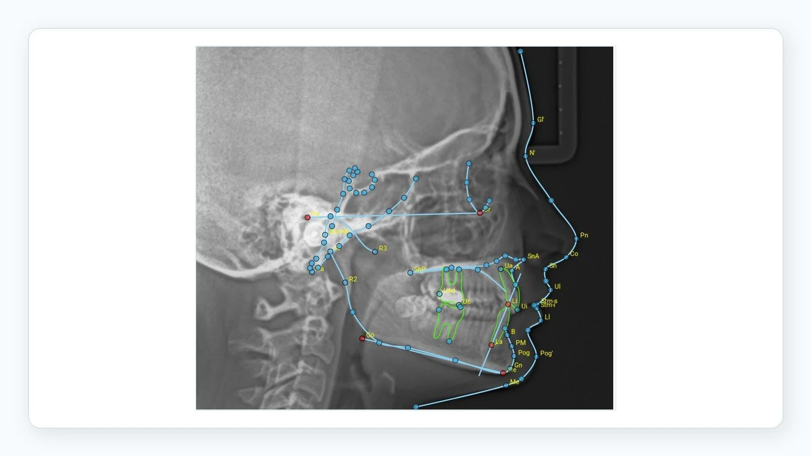
When an orthodontist or radiologist traces a cephalogram, they are identifying specific anatomical reference points called landmarks, then connecting them to form planes, lines, and angles. Think of it as placing GPS pins on a map, then measuring the distances and angles between them. 

Landmarks fall into two categories — hard tissue (bone and dentition) and soft tissue (lips, nose, chin profile) — and the distinction matters because orthodontics has increasingly moved toward treating the whole face, not just the teeth. 

Hard Tissue Landmarks 

These are the bony and dental reference points that form the mathematical skeleton of the analysis. The clinically critical ones are: 

• Sella (S) — The midpoint of the sella turcica, the bony fossa at the skull base that houses the pituitary gland. It serves as the posterior anchor of the cranial base reference line. 

• Nasion (N) — The junction of the nasal and frontal bones at the bridge of the nose. Along with Sella, it forms the SN plane — the most widely used cranial base reference in orthodontics. 

• Point A (Subspinale) — The deepest concavity of the anterior maxillary alveolus, between the anterior nasal spine and the upper incisor. It represents the anterior limit of the upper jaw and is used to calculate SNA and ANB. 

• Point B (Supramentale) — The equivalent concavity in the mandible. Along with Point A, it defines the ANB angle — arguably the single most referenced measurement in orthodontic diagnosis. 

• Pogonion (Pog) — The most anterior point of the bony chin. Used to assess chin projection and mandibular profile. 

• Menton (Me) — The lowest point of the mandibular symphysis. Key for vertical dimension measurements. 

• Gonion (Go) — The posteroinferior angle of the jaw, usually constructed geometrically. Central to mandibular plane analysis and ramus assessment. 

• ANS and PNS — The anterior and posterior nasal spines, which together define the palatal plane: the floor of the nose and roof of the mouth.

Soft Tissue Landmarks 

Soft tissue cephalometrics gained prominence in the 1980s as the profession recognized that skeletal correction alone does not guarantee a good aesthetic outcome. The face the patient presents to the world is soft tissue, and its response to skeletal change is not perfectly predictable. 

• Pronasale — The nasal tip. One anchor of Ricketts' esthetic E-line. 

• Subnasale — The base of the nose where it meets the upper lip. Used for nasolabial angle measurement. 

• Labrale Superius and Inferius — The most prominent points of the upper and lower lips respectively. Their positions relative to the E-line are the standard measure of lip protrusion. 

• Soft Tissue Pogonion — The most anterior point of the soft chin. Used in facial convexity and profile analysis. 

A note on landmark accuracy

Even with digital software, landmark identification is operator-dependent. Two experienced tracers placing the same cephalogram will produce measurement sets that differ by 1–2° for angles and 0.5–1 mm for linear values — this is accepted inter-operator variability, not error. It is why radiologist review of automated landmark detection remains essential in clinical reporting. 

The Three Major Analysis Frameworks

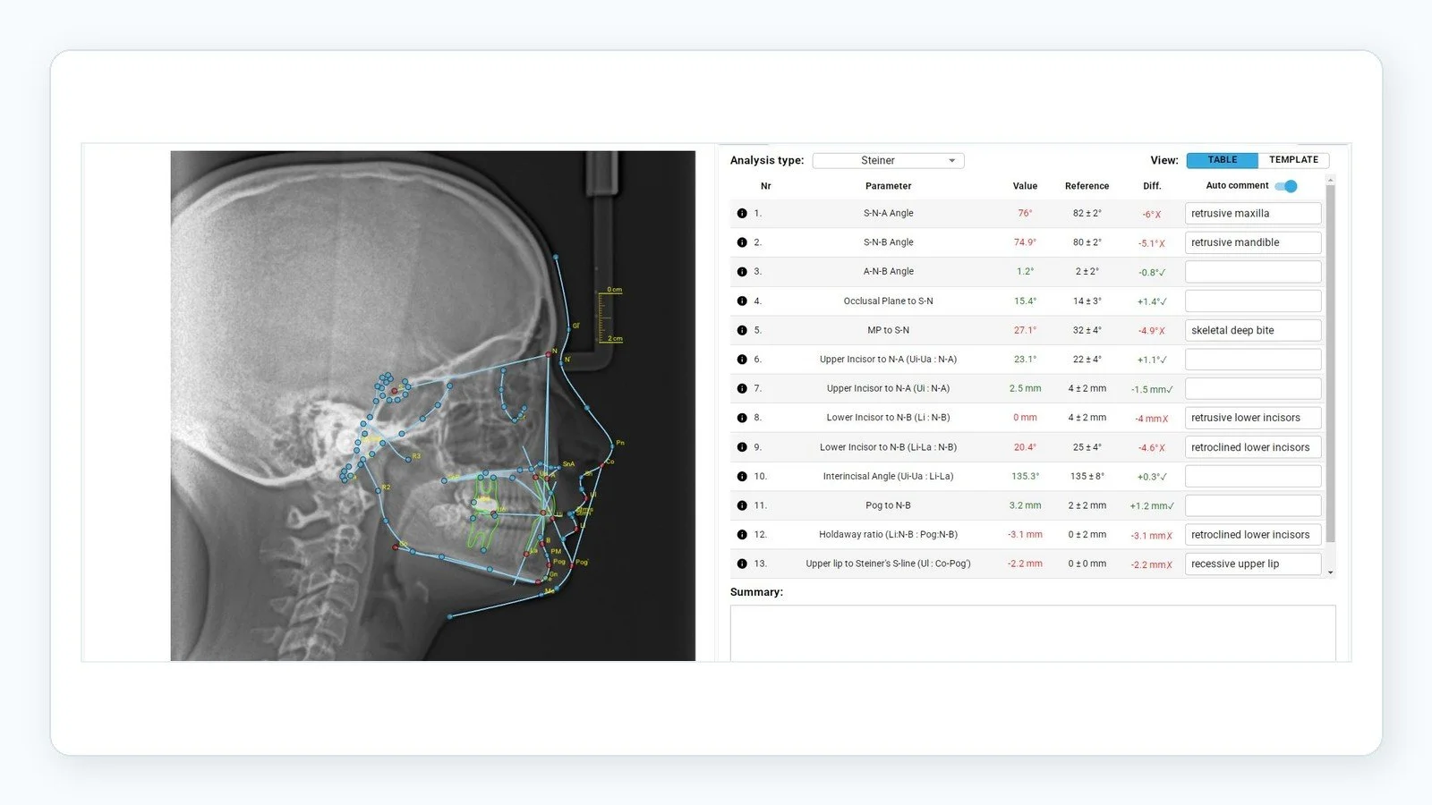
Once landmarks are identified, the measurements are interpreted using an analysis framework — a structured set of norms and reference planes against which the patient's values are compared. The choice of framework often reflects where the orthodontist trained, what clinical question is being asked, and what the software defaults to. Here are the three most widely used systems. 

Steiner Analysis 

Developed by Cecil Steiner in the 1950s and still the most widely taught analysis in dental schools, Steiner uses the Sella-Nasion (SN) line as its primary reference plane. Its central measurements — SNA, SNB, and ANB — have become the universal shorthand for describing jaw relationships. 

SNA (82° ± 2°) measures how far forward the maxilla sits relative to the cranial base. Above 84° suggests a prognathic upper jaw; below 80° indicates retrusion. 

SNB (80° ± 2°) the same measurement for the mandible. A low SNB is the skeletal signature of a receded lower jaw and contributing chin. 

ANB (ideally 1°–3°) the arithmetic difference between SNA and SNB. This single number defines skeletal class: above 4° is Class II (upper jaw forward), zero or negative is Class III (lower jaw forward or equal). 

Upper incisor to NA (22° / 4 mm) the angular inclination and millimeter position of the upper front teeth to the NA line. This guides retraction or proclination decisions. 

Lower incisor to NB (25° / 4 mm) is the equivalent for the lower incisors. High values indicate flared lower front teeth — a key factor in extraction planning. 

Interincisal angle (~130°) the angle between the long axes of the upper and lower central incisors. Below 120° is a reliable indicator of proclined, bimaxillary protruded dentition. 

ANB is probably the most quoted single number in orthodontics. Its elegance is its simplicity — one angle that tells you whether the upper jaw is ahead of, behind, or level with the lower jaw.

Tweed Analysis 

Charles Tweed developed his analysis in the 1940s around what he called the Tweed Triangle — the geometric relationship between three planes: the Frankfort Horizontal (FH), the mandibular plane (MP), and the long axis of the lower central incisor. His framework is built on the premise that the lower incisor should be positioned correctly over its basal bone, and that vertical facial pattern governs how much correction is biologically stable. 

FMA — Frankfort-Mandibular Plane Angle (22°–28°) measures the steepness of the lower jaw. This is the primary indicator of facial type. A high FMA means a steep, hyperdivergent pattern — prone to open bites and less favorable biomechanics. A low FMA is a hypodivergent, deep-bite type. 

IMPA — Incisor-Mandibular Plane Angle (~87°) the inclination of the lower incisor to the mandibular plane. High values indicate proclined lower incisors. 

FMIA — Frankfort-Mandibular Incisor Angle (~68°) Tweed used this as his treatment anchor. He believed extraction decisions should be driven by the need to position the lower incisor correctly over basal bone, and FMIA captures this relationship. 

→  Why FMA matters in clinical practice

High FMA cases — steep mandibular planes — require careful mechanics to avoid further vertical opening, which risks anterior open bite and relapse. Understanding facial type from the FMA changes appliance selection, anchorage planning, and patient prognosis conversations. It is one of the first things an experienced clinician looks at. 

McNamara Analysis 

James McNamara introduced his analysis in 1984 and it represented a genuine conceptual shift. Rather than relying on angular measurements, McNamara used linear distances — millimeters — referenced perpendicular lines dropped from Nasion to the Frankfort Horizontal. The reasoning: a 4 mm discrepancy is more intuitive to visualize and communicate than a 2° angular deviation, and linear measurements have a more direct relationship to surgical planning. 

Maxilla to Nasion Perpendicular – A Point should fall on or within a millimeter of this perpendicular in an average adult. Anterior deviation indicates maxillary protrusion; posterior indicates retrusion. 

Mandible to Nasion Perpendicular - Pogonion position relative to the same perpendicular. In adults, a range of -8 mm to 0 mm (females) and -4 mm to +2 mm (males) is accepted. 

Effective maxillary and mandibular length - Linear measurements from Condylion to Point A (upper jaw) and Condylion to Gnathion (lower jaw). These tell you whether a Class II or III problem stems from a short jaw, a long jaw, or a positioning issue — a distinction that is critical when considering surgery. 

Lower anterior face height (ANS–Menton) - Compared against upper face height to assess vertical proportions. Discrepancies here flag open-bite or deep-bite skeletal tendencies before the clinician even looks at the teeth. 

McNamara's analysis is the framework of choice for surgical orthodontic planning, and most practices that handle complex combined cases will use it alongside Steiner. At DMD Imaging, our reports include both, when indicated. 

Choosing the Right Framework or Combining Them 

In practice, experienced clinicians rarely use a single analysis in isolation. Steiner gives you the skeletal class and incisor positions. Tweed gives you the vertical pattern and a biomechanical rationale. McNamara gives you absolute jaw sizes and the surgical roadmap. Used together, they create a complete diagnostic picture.

	Reference Plane	Measurement Type	Best For
Steiner	Sella-Nasion (SN)	Angular + linear	Skeletal class, incisor inclination, everyday diagnosis
Tweed	Frankfort Horizontal (FH)	Angular (triangle)	Vertical pattern, facial type, extraction rationale
McNamara	Nasion Perpendicular	Linear only	Jaw size vs position, surgical planning

The Digital Tracing Workflow

The days of tracing acetate paper over a light box are largely behind us. What once took a careful clinician 45 minutes — with the attendant risk of eye fatigue and cumulative measurement error — now happens in a structured digital workflow. Here is what that looks like in practice. 

Step 1 — Image acquisition.  The patient is positioned in the cephalostat with the Frankfort Horizontal parallel to the floor, or in natural head position depending on protocol. Ear rods stabilise the head. A digital sensor (flat-panel detector or phosphor plate) captures the image in seconds at approximately 80–90 kVp and 8–12 mA. The radiation dose is around 5–6 microsieverts — roughly equivalent to 30 minutes of natural background radiation, or less than 1% of a standard chest X-ray. 

Step 2 — Image processing.  Once acquired, window and level adjustments optimise both bony landmark visibility and soft tissue contour in the same image — a balance that was genuinely difficult to achieve with analogue film. At DMD Imaging, every image is processed by our radiographers before it reaches the tracing stage. 

Step 3 — Landmark identification.  This is where clinical expertise matters most. Using cephalometric software — commonly Dolphin Imaging, Nemoceph, or OnyxCeph — the operator identifies each landmark in sequence. Semi-automatic detection algorithms suggest positions, but human oversight is non-negotiable. A misplaced Gonion, for example, cascades into errors across the mandibular plane, FMA, and condylar measurements simultaneously. 

Step 4 — Analysis generation.  Once landmarks are confirmed, the software calculates all measurements instantly, compares them against age- and sex-matched normative data, and flags deviations. Multiple analysis frameworks are generated simultaneously — Steiner, Tweed, McNamara, Ricketts, Wits appraisal — in seconds. 

Step 5 — Radiologist review and report delivery.  At DMD Imaging, every tracing is reviewed by a dental radiologist before the report is released. The final document includes the traced image with landmark labels, a tabulated measurement set, narrative interpretation of skeletal and dental findings, soft tissue analysis, growth assessment where requested. Standard turnaround is 24 hours; urgent surgical cases are turned around in 4–6 hours. 

✓  Why radiologist review matters on digital reports

Automated software is efficient and increasingly accurate on well-positioned, artefact-free images. But it cannot assess image quality, flag incidental findings, contextualise measurements against population norms, or recommend a retake. A radiologist can — and at DMD Imaging, every report carries that clinical accountability. 

Ceph vs. CBCT: The Honest Clinical Answer

With cone beam CT (CBCT) units now more accessible across dental practices, a question comes up regularly in clinical conversations: does the conventional lateral cephalogram still have a place, or has 3D imaging made it redundant? 

The honest answer is that the conventional ceph remains the standard of care for routine orthodontic records — and CBCT, while genuinely superior for specific clinical questions, is not a substitute for the 2D cephalogram in most situations. Here is why.

The case for the conventional cephalogram 

• Radiation dose. A digital lateral cephalogram delivers approximately 5–6 microsieverts. A limited-field CBCT for orthodontics delivers 40–130 microsieverts — six to twenty-five times higher. For a growing child who may need serial imaging over several years, this difference is clinically meaningful. 

• Normative data. Every published cephalometric norm — Steiner, Tweed, McNamara, Ricketts, Bolton — is based on conventional 2D cephalograms. There is no equivalent normative database validated for 3D CBCT-derived measurements. Applying 2D analyses to CBCT-generated pseudo-lateral images introduces methodological inconsistency. 

• Cost. A lateral cephalogram is a fraction of the cost of a CBCT. For patients who need multiple sets of records over a multi-year treatment, this matters. 

• Workflow. Most orthodontic software is built around 2D cephalometric inputs. Integrating CBCT into a standard tracing workflow requires additional processing time and software investment that is rarely justified for routine cases. 

When CBCT genuinely changes the diagnosis 

There are specific scenarios where a conventional cephalogram is inadequate and CBCT provides information that meaningfully changes the treatment plan: 

• Impacted canines and supernumerary teeth — CBCT provides precise 3D localisation, buccal vs palatal position, and proximity to adjacent roots that a 2D film cannot. 

• Skeletal asymmetry assessment — Conventional cephalograms project the right and left sides onto one another, masking transverse discrepancies. CBCT allows genuine 3D evaluation of condylar position, ramus height asymmetry, and true midline deviation. 

• Airway assessment — Volumetric measurement of the upper airway is only possible with CBCT, making it essential for patients with sleep-disordered breathing or when orthognathic surgery is being planned. 

• Temporomandibular joint evaluation — High-resolution CBCT shows condylar morphology, cortical integrity, and joint space that 2D imaging cannot provide. 

• Orthognathic surgery planning — Where virtual surgical planning (VSP) will be used, CBCT data is required for 3D osteotomy simulation and surgical splint fabrication. 

→  Our recommendation to referring clinicians

If you are unsure whether a CBCT adds clinical value over a lateral ceph for a specific case, call us before the patient is positioned. Our radiologists routinely advise on appropriate imaging selection — and in the majority of routine orthodontic cases, a high-quality digital cephalogram with an OPG covers everything needed, at a fraction of the dose and cost.

Surgical Orthodontics: How Cephalometrics Guides Jaw Surgery

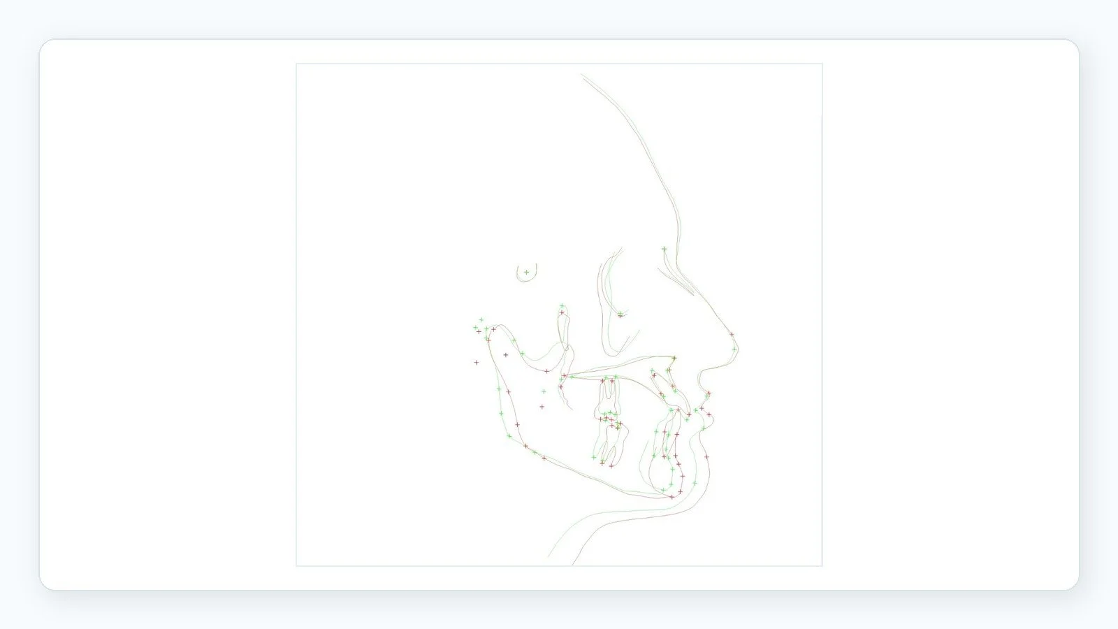
For patients whose skeletal discrepancies exceed what orthodontics alone can address — severe Class II or III jaw relationships, significant anterior open bites, or marked facial asymmetries — the treatment is a combination of orthodontics and orthognathic surgery. Cephalometric analysis is the diagnostic foundation on which this entire plan is built.

What gets determined in the planning phase 

Using McNamara's framework as the primary tool, the orthodontist and oral surgeon together establish which jaw requires movement, in which direction, and by how much. The critical decisions are: 

• Whether to move the maxilla, the mandible, or both — a decision driven by McNamara's effective jaw length measurements, which distinguish a size problem from a position problem. 

• The expected soft tissue response. Upper lip advancement is approximately 60–70% of maxillary advancement. Chin projection changes can be predicted from Pogonion movement. These ratios allow clinicians to anticipate the post-surgical facial profile before a single incision is made. 

• Treatment sequencing — pre-surgical orthodontics to align teeth and remove dental compensations, surgery, then post-surgical finishing. 

From VTO to Virtual Surgical Planning 

The cephalometric prediction tracing — historically called a VTO, or Visualised Treatment Objective — was for decades performed by physically cutting and repositioning acetate tracings to simulate surgical moves. Today, software performs this instantly. But the conceptual underpinning is the same: you need to see the skeletal and soft tissue outcome before operating. 

Modern planning has evolved further into full 3D virtual surgical planning (VSP) using CBCT data — the digital skull is osteotomised on-screen, repositioned, and the resulting splints are milled from the planned positions. For complex cases involving both maxillary and mandibular movements, or significant asymmetries, VSP has become the standard. But even in these cases, the 2D cephalometric analysis remains the starting point for diagnosis and the reference against which the planned outcome is measured. 

⚠  Timing of post-surgical records

Post-surgical cephalograms should only be taken after oedema has fully resolved — ideally no sooner than three months post-operatively. Images taken earlier will show artificially distorted soft tissue profiles that do not reflect the true outcome, and comparing them against pre-surgical records leads to misleading conclusions. 

Normal Growth Patterns — What Changes as a Child Grows?

Cephalometry is not only a diagnostic snapshot — it is a longitudinal tool. Serial cephalograms taken at key intervals allow the clinician to track a child's individual craniofacial growth pattern, predict how untreated discrepancies will evolve, and time interventions to coincide with periods of active growth. 

The direction of mandibular growth 

The mandible grows downward and forward in all individuals, but the proportion of each component varies significantly — and that variation has profound clinical implications. 

• Horizontal (forward) growers tend to develop stronger chins, maintain better facial proportions over time, and are inherently more favourable orthodontic cases. Their FMA is typically below 22°. Results are more stable, open-bite risk is low. 

• Vertical (downward) growers have a steep mandibular plane angle — FMA above 28°. They are prone to anterior open bites, their Class II discrepancies tend to worsen without treatment, and they carry a higher relapse risk. Mechanics that avoid vertical opening are essential for this group. 

• Average growers fall between these extremes, with FMA in the 22–28° range. Most patients are in this category. 

Growth timing and the adolescent spurt 

The adolescent growth spurt — the period of peak craniofacial growth — is the key window for growth modification treatment. In girls, this typically occurs between 10 and 13 years; in boys, between 12 and 15. But chronological age is a rough guide at best. Biological age — assessed through skeletal maturity indicators — is far more reliable. 

The cervical vertebral maturation (CVM) method has become the standard biological marker. The shape and concavity of the C2–C4 vertebrae, visible on the lateral cephalogram, correlate closely with skeletal growth stage. A patient in CVM Stage 3 has approximately 25% of their peak growth remaining. A patient in Stage 5 has largely completed growth. These distinctions change whether a clinician initiates growth modification today, monitors for another year, or moves directly to fixed appliances. 

→  CVM assessment at DMD Imaging

When referring clinicians request growth analysis, our reports include CVM staging based on the cervical vertebrae visible on the lateral cephalogram. This gives the orthodontist a biological growth indicator alongside the standard cephalometric measurements — without requiring an additional hand-wrist X-ray.

Reading Your Cephalometric Report

For patients who have received a cephalometric report and want to understand what the numbers mean — and for clinicians looking for a plain-language translation tool to use with patients — here is what the key measurements are actually telling you.

Measurement	What It Measures	Normal Range	Elevated Value Indicates	Low Value Indicates
SNA	Upper jaw forward position	80°–84°	Prominent upper jaw	Receded upper jaw
SNB	Lower jaw forward position	78°–82°	Prominent lower jaw, strong chin	Receded lower jaw
ANB	Upper vs lower jaw balance	1°–3°	Class II — upper jaw forward	Class III — lower jaw forward
FMA	Jaw angle steepness	22°–28°	Open bite tendency, long face pattern	Deep bite tendency, short face pattern
IMPA	Lower incisor tilt	85°–95°	Flared lower front teeth	Upright or retroclined teeth
Interincisal angle	Upper + lower incisor angle	125°–135°	Upright teeth, less protrusion	Flared / proclined dentition
Upper lip to E-line	Upper lip projection	−4 to 0 mm	Lip protrudes past the line	Lip behind the line — retrusive

✓  The most important thing to understand about your report

A value outside the normal range is not automatically a problem requiring treatment. The same ANB of 5° might be managed with growth modification in a ten-year-old, monitored in a twelve-year-old, treated with orthodontics alone in a sixteen-year-old, or considered for surgery only if it is severe enough to affect function in an adult. Numbers inform the clinical decision — they do not make it. Your orthodontist is interpreting the whole picture, not just the deviations column.

AI-Assisted Analysis — Where It Stands Today 

Artificial intelligence has entered cephalometric landmark detection in a meaningful way. Several platforms now offer fully automated landmark identification and analysis generation — the computer places all points and produces a complete multi-analysis report in under a minute. 

The accuracy on high-quality, well-positioned images is genuinely impressive, with error rates for many landmarks now comparable to experienced human operators. But several limitations are real and worth understanding. 

• Performance degrades significantly with poor image quality, unusual anatomy, presence of orthodontic appliances, or heavy metallic restorations. These are exactly the complex cases where accurate analysis matters most. 

• AI models trained predominantly on Western population datasets show lower accuracy on South and East Asian craniofacial morphology — a practical limitation in the clinical context of most practices in this region. 

• Automated systems cannot flag incidental findings, assess image quality, contextualise measurements against local population norms, or recommend a retake. These require clinical judgement. 

At DMD Imaging, we use AI-assisted landmark detection as a first-pass efficiency tool. Every report is then reviewed and endorsed by a qualified dental radiologist before release. That combination — AI speed with human clinical accountability — is where the technology currently sits at its most reliable.

Why This Still Matters 

In an era of 3D scanning, digital models, AI diagnostics, and intraoral photography, the lateral cephalogram might seem like a relic of mid-twentieth century radiology. It is not. 

It remains the only standardised, normatively validated, low-dose method for measuring facial skeletal structure in a way that is directly comparable across patients, across time, and across the entire published literature. The conceptual framework of cephalometric analysis — the discipline of measuring, contextualising, and communicating craniofacial anatomy — is the foundation on which modern orthodontic and surgical diagnosis rests. Everything else builds from it. 

Whether you are an orthodontist reviewing your fourth ceph of the morning or a patient trying to make sense of the diagram your doctor showed you during consultation, the essential point is the same: this is not just an X-ray. It is a precise, reproducible, clinically actionable measurement of the face. Understanding what it measures is the first step toward understanding your treatment.

✦ Refer to DMD Imaging

→ Lateral cephalometric Tracing & Analysis reviewed by dental radiologists

→ 24-hour standard turnaround · 4–6 hour urgent delivery

→ Steiner, Tweed, McNamara, Ricketts — all frameworks available

→ CVM growth assessment included on request

→ Remote reporting for practices across India — Tier 1, 2, and 3 cities

→ CBCT, OPG, and full orthodontic records packages also available

Frequently Asked Questions

• What is a lateral cephalogram and why does my orthodontist need it before starting treatment?

  A lateral cephalogram is a standardised side-view skull X-ray that lets your orthodontist measure the exact positions and proportions of your upper jaw, lower jaw, teeth, and facial profile. Without it, planning is based only on what the clinician can see inside the mouth. The ceph reveals the skeletal architecture underneath — which determines whether extractions are needed, whether growth modification is appropriate, and whether the case eventually requires surgical correction. It is one of the few investigations that genuinely changes treatment planning, not just confirms it.

• Is the radiation from a cephalometric X-ray safe?

  Yes, comfortably so. A single digital lateral cephalogram delivers approximately 5–6 microsieverts of radiation — equivalent to roughly 30 minutes of normal background radiation from the environment. For comparison, a chest X-ray delivers around 100 microsieverts and a long-haul flight exposes you to approximately 80 microsieverts. Even for growing children who require serial cephalograms over the course of treatment, the cumulative dose remains well within internationally accepted safety limits.

• My report says my ANB is 5°. Does that mean I need jaw surgery?

  Not necessarily. ANB of 5° is a Class II skeletal indicator — it tells the clinician that the upper jaw sits further forward relative to the lower jaw than average. But the same measurement means different things at different ages and in different clinical contexts. In a growing child, it may be corrected with functional appliances during the growth spurt. In an adolescent, it can often be managed with fixed orthodontics and appropriate mechanics. Surgery is considered only when the discrepancy is severe enough that orthodontic treatment alone cannot achieve acceptable function and aesthetics. One number does not determine a treatment plan.

• What does a 'high FMA' mean, and why does my orthodontist keep mentioning it?

  FMA — the Frankfort-Mandibular Plane Angle — measures the steepness of your lower jaw. A high FMA (above 28°) means your lower jaw is angled steeply downward, which is associated with a longer lower face, a tendency toward anterior open bite, and more challenging biomechanics during treatment. Orthodontists treat high-FMA cases carefully because mechanics that allow vertical opening can worsen the facial pattern and increase relapse risk. If your doctor is mentioning your FMA, it likely means your treatment mechanics are being selected specifically to manage this tendency — which is the right approach.

• How do I get a cephalometric report from DMD Imaging if I'm in a smaller city?

  We offer remote reporting for practices across India. You submit DICOM images captured on your in-house sensor through our referring clinician portal and receive a full radiologist-reviewed report within 24 hours. This service was specifically designed for practices where specialist dental radiology expertise is not available locally. Urgent cases — surgical planning, time-sensitive consultations — are turned around in 4–6 hours. Contact our team for referring clinician registration and onboarding.

• The report mentions 'bimaxillary protrusion' — what does that mean and is it serious?

  Bimaxillary protrusion means both the upper and lower front teeth and their supporting bone are positioned more forward than the average norm. It presents as a fuller, more prominent lip profile and is a common finding across populations in South and Southeast Asia. Whether it requires treatment depends entirely on the patient's concerns and the functional situation — many people with this profile have a perfectly healthy, functional bite and are entirely comfortable with their appearance. It becomes an orthodontic priority only when the patient wants to reduce lip prominence or when the incisor inclination is contributing to crowding, spacing, or soft tissue tension. It is a trait, not a diagnosis requiring automatic correction.